
lavaan簡明教程 [中文翻譯版] 譯者註:此文檔原作者為比利時Ghent大學的Yves Rosseel博士,lavaan亦為其開發,完全開源、免費。我在學習的時候順手翻譯了一下,向Yves的開源精神致敬。此翻譯因偷懶部分刪減,但也有增加,有錯誤請留言 「轉載請註明出處」 目錄 lavaan簡明教 ...
lavaan簡明教程 [中文翻譯版]
譯者註:此文檔原作者為比利時Ghent大學的Yves Rosseel博士,lavaan亦為其開發,完全開源、免費。我在學習的時候順手翻譯了一下,向Yves的開源精神致敬。此翻譯因偷懶部分刪減,但也有增加,有錯誤請留言
「轉載請註明出處」
目錄
lavaan簡明教程 [中文翻譯版]
目錄
摘要
- 在開始之前
- 安裝lavaan包
- 模型語法
- 例1:驗證性因數分析(CFA)
- 例2:結構方程(SEM)
- 更多關於語法的內容
6.1 固定參數
6.2 初值
6.3 參數標簽
6.4 修改器
6.5 簡單相等約束
6.6 非線性相等和不相等約束 - 引入平均值
- 結構方程的多組分析
8.1 在部分組中固定參數
8.2 約束一個參數使其在各組中相等
8.3 約束一組參數使其在各組中相等
8.4 測量不變性 - 增長曲線模型
- 使用分類變數
- 將協方差矩陣作為輸入
- 估計方法,標準誤差和缺失值
12.1 估計方法
12.2 最大似然估計
12.3 缺失值 - 間接效應和中介分析
- 修正指標
- 從擬合方程中提取信息
摘要
此教程首先介紹lavaan的基本組成部分:模型語法,擬合方程(CFA, SEM和growth),用來呈現結果的主要函數(summary, coef, fitted, inspect);
然後提供兩個實例;
最後再討論一些重要話題:均值結構模型(meanstructures),多組模型(multiple groups),增長曲線模型(growth curve models),中介分析(mediation analysis),分類數據(categorial data)等。
1. 在開始之前
在開始之前,有以下幾點需要註意:
- lavaan包需要安裝 3.0.0或更新版本的R。
- lavaan包仍處於未完成階段,目前尚未實現的功能有:對多層數據的支持,對離散潛變數的支持,貝葉斯估計。
- 雖然目前是測試版,但是結果精確,語法成熟,可以放心使用。
- lavaan包對R語言預備知識要求很低。
- 此教程不等於參考手冊,相關文檔正在準備。
- lavaan包是完全免費開源的軟體,不做任何承諾。
- 發現bug,到 https://groups.google.com/d/forum/lavaan/ 加組溝通。
2. 安裝lavaan包
啟動R,並輸入:
install.packages("lavaan", dependencies = TRUE)  # 安裝lavaan包
library(lavaan)   # 載入lavaan包
出現以下提示,表示載入成功。
3. 模型語法
lavaan包的核心是描述整個模型的“模型語法”。這部分簡單介紹語法,更多細節在接下來的示例中可見。
R環境下的回歸方程有如下形式:
y ~ x1 + x2 + x3 + x4 # ~左邊為因變數y在lavaan中,一個典型模型是一個回歸方程組,其中可以包含潛變數,例如:
y ~ f1 + f2 + x1 + x2
f1 ~ f2 + f3
f2 ~ f3 + x1 + x2我們必須通過指示符=~(measured by)來“定義”潛變數。例如,通過以下方式來定義潛變數f1, f2和f3:
f1 =~ y1 + y2 + y3
f2 =~ y4 + y5 + y6
f3 =~ y7 + y8 + y9 + y10
方差和協方差表示如下:
y1 ~~ y1 # 方差
y1 ~~ y2 # 協方差
f1 ~~ f2 # 協方差
只有截距項的回歸方程表達如下:
y1 ~ 1
f1 ~ 1以上4種公式種類(~, ~~, =~, ~ 1)組合成完整的模型語法,用單引號表示如下:
myModel <- ' # 主要回歸方程
             y1 + y2 ~ f1 + f2 + x1 + x2
                  f1 ~ f2 + f3
                  f2 ~ f3 + x1 + x2

             # 定義潛變數
             f1 =~ y1 + y2 + y3
             f2 =~ y4 + y5 + y6
             f3 =~ y7 + y8 + y9 + y10

             # 方差和協方差
             y1 ~~ y1
             y1 ~~ y2
             f1 ~~ f2

             # 截距項
             y1 ~ 1
             f1 ~ 1
如果模型很長,可以將模型(單引號之間的內容)儲存入myModel.lav的txt文檔中,用以下命令讀取:
myModel <- readLines("/mydirectory/myModel.lav") # 這裡需要絕對路徑4. 例1:驗證性因數分析(CFA)
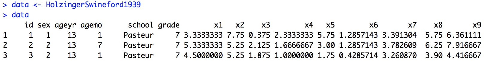
lavaan包提供了一個內置數據集叫做HolzingerSwineford,輸入以下命令查看數據集描述:
?HolzingerSwineford數據形式是這樣的:
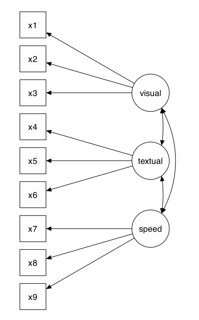
此數據集包含了來自兩個學校的七、八年級孩子的智力能力測驗分數。在我們的版本里,只包含原有26個測試中的9個,這9個測試分數作為9個測量變數分別對應3個潛變數:
- 視覺因數(visual)對應x1,x2,x3
- 文本因數(textual)對應x4,x5,x6
- 速度因數(speed)對應x7,x8,x9
模型如下圖所示:
建立模型代碼如下:
HS.model <- ' visual  =~ x1 + x2 + x3
              textual =~ x4 + x5 + x6
              speed   =~ x7 + x8 + x9'
# 然後擬合cfa函數,第一個參數是模型,第二個參數是數據集
fit <- cfa(HS.model, data = HolzingerSwineford1939)
# 再通過summary函數給出結果
summary(fit, fit.measure = TRUE)
結果展示如下:
# 前6行為頭部,包含版本號,收斂情況,迭代次數,觀測數,用來計算參數的估計量,模型檢驗統計量,自由度和相關的p值
lavaan (0.5-23.1097) converged normally after  35 iterations

  Number of observations                           301

  Estimator                                         ML
  Minimum Function Test Statistic               85.306
  Degrees of freedom                                24
  P-value (Chi-square)                           0.000

#參數fit.measure = TRUE會顯示下麵從model test baseline model到SRMR的部分
Model test baseline model:

  Minimum Function Test Statistic              918.852
  Degrees of freedom                                36
  P-value                                        0.000

User model versus baseline model:

  Comparative Fit Index (CFI)                    0.931
  Tucker-Lewis Index (TLI)                       0.896

Loglikelihood and Information Criteria:

  Loglikelihood user model (H0)              -3737.745
  Loglikelihood unrestricted model (H1)      -3695.092

  Number of free parameters                         21
  Akaike (AIC)                                7517.490
  Bayesian (BIC)                              7595.339
  Sample-size adjusted Bayesian (BIC)         7528.739

Root Mean Square Error of Approximation:

  RMSEA                                          0.092
  90 Percent Confidence Interval          0.071  0.114
  P-value RMSEA <= 0.05                          0.001

Standardized Root Mean Square Residual:

  SRMR                                           0.065

#以下是參數估計部分
Parameter Estimates:

  Information                                 Expected
  Standard Errors                             Standard

Latent Variables:
                   Estimate  Std.Err  z-value  P(>|z|)
  visual =~
    x1                1.000
    x2                0.554    0.100    5.554    0.000
    x3                0.729    0.109    6.685    0.000
  textual =~
    x4                1.000
    x5                1.113    0.065   17.014    0.000
    x6                0.926    0.055   16.703    0.000
  speed =~
    x7                1.000
    x8                1.180    0.165    7.152    0.000
    x9                1.082    0.151    7.155    0.000

Covariances:
                   Estimate  Std.Err  z-value  P(>|z|)
  visual ~~
    textual           0.408    0.074    5.552    0.000
    speed             0.262    0.056    4.660    0.000
  textual ~~
    speed             0.173    0.049    3.518    0.000

Variances:
                   Estimate  Std.Err  z-value  P(>|z|)
   .x1                0.549    0.114    4.833    0.000
   .x2                1.134    0.102   11.146    0.000
   .x3                0.844    0.091    9.317    0.000
   .x4                0.371    0.048    7.779    0.000
   .x5                0.446    0.058    7.642    0.000
   .x6                0.356    0.043    8.277    0.000
   .x7                0.799    0.081    9.823    0.000
   .x8                0.488    0.074    6.573    0.000
   .x9                0.566    0.071    8.003    0.000
    visual            0.809    0.145    5.564    0.000
    textual           0.979    0.112    8.737    0.000
    speed             0.384    0.086    4.451    0.000
例1是一個定義模型、擬合模型、提取結果的過程。
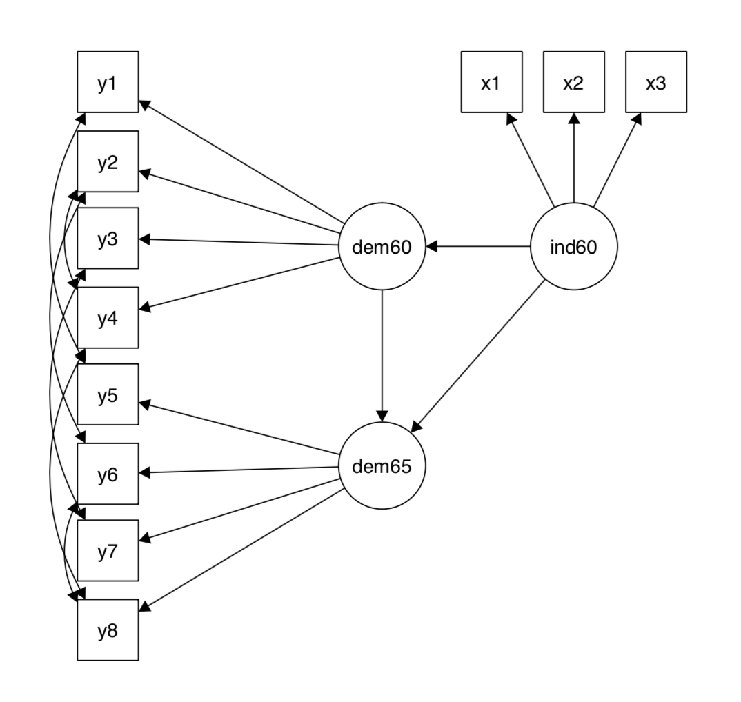
5. 例2:結構方程(SEM)
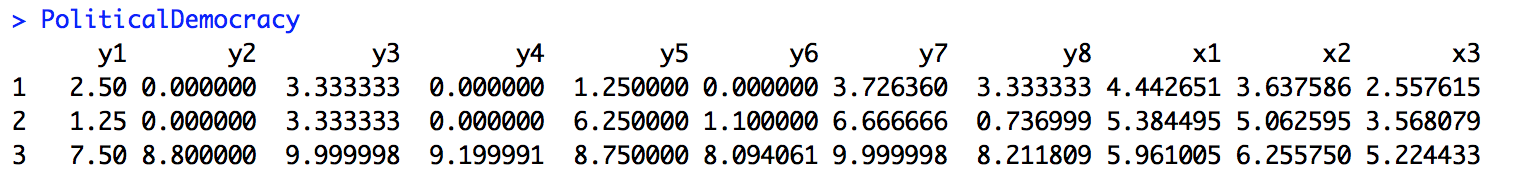
例2中我們使用名為PoliticalDemocracy的數據集,圖示如下:
數據形式大致如下(只顯示前三行):
| 變數 | 含義 | 變數 | 含義 |
|---|---|---|---|
| ind60 | 1960年的非民主情況 | y5 | 1965年專家對出版物自由的評價 |
| dem60 | 1960年的民主情況 | y6 | 1965年的反對黨派自由 |
| dem65 | 1965年的民主情況 | y7 | 1965年選舉的公平性 |
| y1 | 1960年專家對出版物自由的評價 | y8 | 1965年選舉產生的立法機關效率 |
| y2 | 1960年的反對黨派自由 | x1 | 1960年每單位資本GNP |
| y3 | 1960年選舉的公平性 | x2 | 1960年每單位資本的物質能量消費 |
| y4 | 1960年選舉產生的立法機關效率 | x3 | 1960年工業勞動力占比 |
模型如下:
model <- '# measurement model 測量模型
          ind60 =~ x1 + x2 + x3
          dem60 =~ y1 + y2 + y3 + y4
          dem65 =~ y5 + y6 + y7 + y8

          # regressions 回歸
          dem60 ~ ind60
          dem65 ~ ind60 + dem60

          # residual correlations 殘餘相關
          y1 ~~ y5
          y2 ~~ y4 + y6
          y3 ~~ y7
          y4 ~~ y8
          y6 ~~ y8'

# 擬合SEM
fit <- sem(model, data = PoliticalDemocracy)

# 提取結果
summary(fit, standardized = TRUE)

#與上例不同,這裡我們忽略了參數fit.measure = TRUE,用standardized = TRUE來標準化參數值)
結果如下:
lavaan (0.5-23.1097) converged normally after  68 iterations

  Number of observations                            75

  Estimator                                         ML
  Minimum Function Test Statistic               38.125
  Degrees of freedom                                35
  P-value (Chi-square)                           0.329

Parameter Estimates:

  Information                                 Expected
  Standard Errors                             Standard

Latent Variables:
                   Estimate  Std.Err  z-value  P(>|z|)   Std.lv  Std.all
  ind60 =~
    x1                1.000                               0.670    0.920
    x2                2.180    0.139   15.742    0.000    1.460    0.973
    x3                1.819    0.152   11.967    0.000    1.218    0.872
  dem60 =~
    y1                1.000                               2.223    0.850
    y2                1.257    0.182    6.889    0.000    2.794    0.717
    y3                1.058    0.151    6.987    0.000    2.351    0.722
    y4                1.265    0.145    8.722    0.000    2.812    0.846
  dem65 =~
    y5                1.000                               2.103    0.808
    y6                1.186    0.169    7.024    0.000    2.493    0.746
    y7                1.280    0.160    8.002    0.000    2.691    0.824
    y8                1.266    0.158    8.007    0.000    2.662    0.828

Regressions:
                   Estimate  Std.Err  z-value  P(>|z|)   Std.lv  Std.all
  dem60 ~
    ind60             1.483    0.399    3.715    0.000    0.447    0.447
  dem65 ~
    ind60             0.572    0.221    2.586    0.010    0.182    0.182
    dem60             0.837    0.098    8.514    0.000    0.885    0.885

Covariances:
                   Estimate  Std.Err  z-value  P(>|z|)   Std.lv  Std.all
 .y1 ~~
   .y5                0.624    0.358    1.741    0.082    0.624    0.296
 .y2 ~~
   .y4                1.313    0.702    1.871    0.061    1.313    0.273
   .y6                2.153    0.734    2.934    0.003    2.153    0.356
 .y3 ~~
   .y7                0.795    0.608    1.308    0.191    0.795    0.191
 .y4 ~~
   .y8                0.348    0.442    0.787    0.431    0.348    0.109
 .y6 ~~
   .y8                1.356    0.568    2.386    0.017    1.356    0.338

Variances:
                   Estimate  Std.Err  z-value  P(>|z|)   Std.lv  Std.all
   .x1                0.082    0.019    4.184    0.000    0.082    0.154
   .x2                0.120    0.070    1.718    0.086    0.120    0.053
   .x3                0.467    0.090    5.177    0.000    0.467    0.239
   .y1                1.891    0.444    4.256    0.000    1.891    0.277
   .y2                7.373    1.374    5.366    0.000    7.373    0.486
   .y3                5.067    0.952    5.324    0.000    5.067    0.478
   .y4                3.148    0.739    4.261    0.000    3.148    0.285
   .y5                2.351    0.480    4.895    0.000    2.351    0.347
   .y6                4.954    0.914    5.419    0.000    4.954    0.443
   .y7                3.431    0.713    4.814    0.000    3.431    0.322
   .y8                3.254    0.695    4.685    0.000    3.254    0.315
    ind60             0.448    0.087    5.173    0.000    1.000    1.000
   .dem60             3.956    0.921    4.295    0.000    0.800    0.800
   .dem65             0.172    0.215    0.803    0.422    0.039    0.039
可以看出sem()和cfa()這兩個函數很相似,實際上,這兩個函數現在幾乎是一樣的,但在將來可能發生變化。
在添加了standardized參數後,出現了Std.lv, Std.all兩列,前者只有潛變數被標準化了,後者為所有變數都標準化了,也被稱為“完全標準化解”。
6. 更多關於語法的內容
6.1 固定參數
對於一個對應4個指標的潛變數,lavaan預設將第一個指標的因數載荷固定為1,其他指標為自由。
但如果你有一個很好的理由來讓所有因數載荷都固定為1,可以照如下做法:
f =~ y1 + 1*y2 + 1*y3 + 1*y4一般來說,你需要通過給相關變數預先乘以一個數字來固定公式的參數,這個叫做“預乘機制”。
回想例1中的模型,預設3個潛變數兩兩相關。如果你想將某對變數的相關係數設為0,你需要為其添加一個協方差公式並將參數設為0.
在下麵的語法中,除visual,textual間的協方差自由外,其他均設為0。並且我們希望固定speed的因數為一個單位,所以不需要設定第一個指標x7為1,因此我們給x7乘以NA使x7的因數載荷自由且未知,整個模型如下:
# three-factor model
  visual  =~ x1 + x2 + x3
  textual =~ x4 + x5 + x6
  speed   =~ NA*x7 + x8 + x9

# orthogonal factors 正交因數
  visual  ~~ 0*speed
  textual ~~ 0*speed

# fix variance of speed factor
  speed ~~ 1*speed
你也可以用orthogonal = TRUE參數使所有潛變數正交,操作如下:
HS.model <- 'visual  =~ x1 + x2 + x3
             textual =~ x4 + x5 + x6
             speed   =~ x7 + x8 + x9'

fit.HS.ortho <- cfa(HS.model, data = HolzingerSwineford1939, orthogonal = TRUE)
相似的,你可以用std.lv = TRUE使所有潛變數的方差固定為一個單位:
HS.model <- 'visual  =~ x1 + x2 + x3
             textual =~ x4 + x5 + x6
             speed   =~ x7 + x8 + x9'

fit <- cfa(HS.model, data = HolzingerSwineford1939, std.lv = TRUE)
6.2 初值
lavaan包預設為自由參數自動生成初值,你也可以通過start()函數來自己設定初值,示例如下:
visual  =~ x1 + start(0.8)*x2 + start(1.2)*x3
textual =~ x4 + start(0.5)x5 + start(1.0)x6
speed   =~ x7 + start(0.7)x8 + start(1.8)x9
6.3 參數標簽
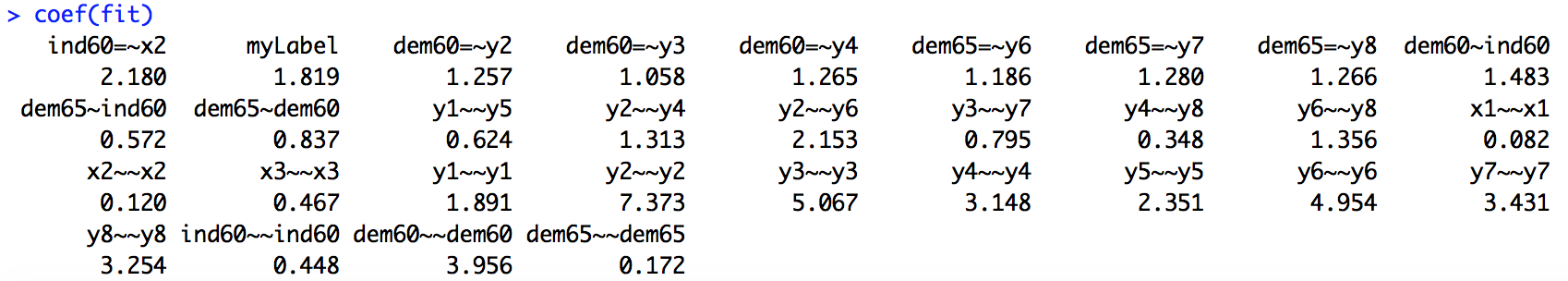
我們也可以自己定義參數標簽,標簽不能以數字開頭:
model <- '
  # latent variable definitions
    ind60 =~ x1 + x2 + myLabel*x3   #將ind60 =~ x3顯示為myLabel
    dem60 =~ y1 + y2 + y3 + y4
    dem65 =~ y5 + y6 + y7 + y8
  # regressions
    dem60 ~ ind60
    dem65 ~ ind60 + dem60
  # residual (co)variances
    y1 ~~ y5
    y2 ~~ y4 + y6
    y3 ~~ y7
    y4 ~~ y8
    y6 ~~ y8'

fit <- sem(model,
           data = PoliticalDemocracy)
coef(fit)
結果如下:
6.4 修改器
我們預乘機制所使用的固定參數,修改初始值和參數標簽等操作,都可以稱為修改器,比如:
f =~ y1 + y2 + myLabel*y3 + start(0.5)*y3 + y4
#雖然y3項出現了兩次,過濾器仍然會將y3作為一個指標對待
6.5 簡單相等約束
有些情況我們會預設變數參數相等,可以用相同的label達到效果,也可以用equal()函數:
visual  =~ x1 + v2*x2 + v2*x3
textual =~ x4 + x5 + x6
speed   =~ x7 + x8 + x9

#或者用equal()
visual  =~ x1 + x2 + equal("visual=~x2")*x3
textual =~ x4 + x5 + x6
speed   =~ x7 + x8 + x9
6.6 非線性相等和不相等約束
假設有如下回歸方程:
y ~ b1*x1 + b2*x2 + b3*x3我們用隨機數生成一個數據集,並用sem函數擬合:
set.seed(1234)
Data <- data.frame(y = rnorm(100),
                   x1 = rnorm(100),
                   x2 = rnorm(100),
                   x3 = rnorm(100))
model <- 'y ~ b1*x1 + b2*x2 + b3*x3'
fit <- sem(model, data = Data)
coef(fit)
結果為:
    b1     b2     b3   y~~y
-0.052  0.084  0.139  0.970
如果我們想要為b1增加兩個約束:\(b_1=(b_2+b_3)^2\) 和 \(b_1\ge\exp(b_2+b_3)\),操作如下:
model.constr <- '# model with labeled parameters
                 y ~ b1*x1 + b2*x2 + b3*x3
                 # constraints
                 b1 == (b2 + b3)^2
                 b1 > exp(b2 + b3)'
fit <- sem(model.constr, data = Data)
coef(fit)
結果如下:
    b1     b2     b3   y~~y
 0.495 -0.405 -0.299  1.610
7. 引入平均值
總的來說,結構方程用來模擬指標變數的協方差矩陣,但是在一些應用中,引入指標變數的均值也是有用的。一個方法是求助於截距項,使用如下所示的“截距公式”:
variable ~ 1右邊的1代表截距,比如在例1中,我們可以增加截距項到指標變數中:
# three-factor model
  visual  =~ x1 + x2 + x3
  textual =~ x4 + x5 + x6
  speed   =~ x7 + x8 + x9
# intercepts
  x1 ~ 1
  x2 ~ 1
  x3 ~ 1
  x4 ~ 1
  x5 ~ 1
  x6 ~ 1
  x7 ~ 1
  x8 ~ 1
  x9 ~ 1
然而還有一種更簡單的方法:
fit <- cfa(HS.model,
           data = HolzingerSwineford1939,
           meanstructure = TRUE)
summary(fit)
結果如下:
lavaan (0.5-23.1097) converged normally after  35 iterations

  Number of observations                           301

  Estimator                                         ML
  Minimum Function Test Statistic               85.306
  Degrees of freedom                                24
  P-value (Chi-square)                           0.000

Parameter Estimates:

  Information                                 Expected
  Standard Errors                             Standard

Latent Variables:
                   Estimate  Std.Err  z-value  P(>|z|)
  visual =~
    x1                1.000
    x2                0.554    0.100    5.554    0.000
    x3                0.729    0.109    6.685    0.000
  textual =~
    x4                1.000
    x5                1.113    0.065   17.014    0.000
    x6                0.926    0.055   16.703    0.000
  speed =~
    x7                1.000
    x8                1.180    0.165    7.152    0.000
    x9                1.082    0.151    7.155    0.000

Covariances:
                   Estimate  Std.Err  z-value  P(>|z|)
  visual ~~
    textual           0.408    0.074    5.552    0.000
    speed             0.262    0.056    4.660    0.000
  textual ~~
    speed             0.173    0.049    3.518    0.000

Intercepts:
                   Estimate  Std.Err  z-value  P(>|z|)
   .x1                4.936    0.067   73.473    0.000
   .x2                6.088    0.068   89.855    0.000
   .x3                2.250    0.065   34.579    0.000
   .x4                3.061    0.067   45.694    0.000
   .x5                4.341    0.074   58.452    0.000
   .x6                2.186    0.063   34.667    0.000
   .x7                4.186    0.063   66.766    0.000
   .x8                5.527    0.058   94.854    0.000
   .x9                5.374    0.058   92.546    0.000
    visual            0.000
    textual           0.000
    speed             0.000

Variances:
                   Estimate  Std.Err  z-value  P(>|z|)
   .x1                0.549    0.114    4.833    0.000
   .x2                1.134    0.102   11.146    0.000
   .x3                0.844    0.091    9.317    0.000
   .x4                0.371    0.048    7.779    0.000
   .x5                0.446    0.058    7.642    0.000
   .x6                0.356    0.043    8.277    0.000
   .x7                0.799    0.081    9.823    0.000
   .x8                0.488    0.074    6.573    0.000
   .x9                0.566    0.071    8.003    0.000
    visual            0.809    0.145    5.564    0.000
    textual           0.979    0.112    8.737    0.000
    speed             0.384    0.086    4.451    0.000
如上圖所示,模型包含觀測變數和潛變數的截距參數。lavaan包預設cfa()和sem()函數將潛變數截距固定為0,否則模型不能被估計。要註意的是均值結構模型中卡方統計量和自由度和原方程一樣,原因是我們引入了9個觀測變數的均值,也同時加上了9個額外的結截距參數。新老兩模型的估計結果是完全一樣的。在實踐中,我們增加截距公式的唯一原因是因為一些約束必須被規定。例如,我們必須設定x1,x2,x3,x4的截距都為0.5時,語法如下:
# three-factor model
  visual  =~ x1 + x2 + x3
  textual =~ x4 + x5 + x6
  speed   =~ x7 + x8 + x9
# intercepts with fixed values
  x1 + x2 + x3 + x4 ~ 0.5*1
8. 結構方程的多組分析
lavaan包完全支持多組分析。為了進行多組分析,你需要在數據組中加上組變數的名稱。預設情況下,所有組會擬合相同的模型。在以下示例中,我們針對兩個學校(Pasteur和Grant-White,可以看到數據集中有關學校的變數名為school)擬合例1的模型:
HS.model <- 'visual  =~ x1 + x2 + x3
             textual =~ x4 + x5 + x6
             speed   =~ x7 + x8 + x9'
fit <- cfa(HS.model,
           data = HolzingerSwineford1939,
           group = "school")
summary(fit)
結果如下:
lavaan (0.5-23.1097) converged normally after  57 iterations

  Number of observations per group
  Pasteur                                          156
  Grant-White                                      145

  Estimator                                         ML
  Minimum Function Test Statistic              115.851
  Degrees of freedom                                48
  P-value (Chi-square)                           0.000

Chi-square for each group:

  Pasteur                                       64.309
  Grant-White                                   51.542

Parameter Estimates:

  Information                                 Expected
  Standard Errors                             Standard


Group 1 [Pasteur]:

Latent Variables:
                   Estimate  Std.Err  z-value  P(>|z|)
  visual =~
    x1                1.000
    x2                0.394    0.122    3.220    0.001
    x3                0.570    0.140    4.076    0.000
  textual =~
    x4                1.000
    x5                1.183    0.102   11.613    0.000
    x6                0.875    0.077   11.421    0.000
  speed =~
    x7                1.000
    x8                1.125    0.277    4.057    0.000
    x9                0.922    0.225    4.104    0.000

Covariances:
                   Estimate  Std.Err  z-value  P(>|z|)
  visual ~~
    textual           0.479    0.106    4.531    0.000
    speed             0.185    0.077    2.397    0.017
  textual ~~
    speed             0.182    0.069    2.628    0.009

Intercepts:
                   Estimate  Std.Err  z-value  P(>|z|)
   .x1                4.941    0.095   52.249    0.000
   .x2                5.984    0.098   60.949    0.000
   .x3                2.487    0.093   26.778    0.000
   .x4                2.823    0.092   30.689    0.000
   .x5                3.995    0.105   38.183    0.000
   .x6                1.922    0.079   24.321    0.000
   .x7                4.432    0.087   51.181    0.000
   .x8                5.563    0.078   71.214    0.000
   .x9                5.418    0.079   68.440    0.000
    visual            0.000
    textual           0.000
    speed             0.000

Variances:
                   Estimate  Std.Err  z-value  P(>|z|)
   .x1                0.298    0.232    1.286    0.198
   .x2                1.334    0.158    8.464    0.000
   .x3                0.989    0.136    7.271    0.000
   .x4                0.425    0.069    6.138    0.000
   .x5                0.456    0.086    5.292    0.000
   .x6                0.290    0.050    5.780    0.000
   .x7                0.820    0.125    6.580    0.000
   .x8                0.510    0.116    4.406    0.000
   .x9                0.680    0.104    6.516    0.000
    visual            1.097    0.276    3.967    0.000
    textual           0.894    0.150    5.963    0.000
    speed             0.350    0.126    2.778    0.005


Group 2 [Grant-White]:

Latent Variables:
                   Estimate  Std.Err  z-value  P(>|z|)
  visual =~
    x1                1.000
    x2                0.736    0.155    4.760    0.000
    x3                0.925    0.166    5.583    0.000
  textual =~
    x4                1.000
    x5                0.990    0.087   11.418    0.000
    x6                0.963    0.085   11.377    0.000
  speed =~
    x7                1.000
    x8                1.226    0.187    6.569    0.000
    x9                1.058    0.165    6.429    0.000

Covariances:
                   Estimate  Std.Err  z-value  P(>|z|)
  visual ~~
    textual           0.408    0.098    4.153    0.000
    speed             0.276    0.076    3.639    0.000
  textual ~~
    speed             0.222    0.073    3.022    0.003

Intercepts:
                   Estimate  Std.Err  z-value  P(>|z|)
   .x1                4.930    0.095   51.696    0.000
   .x2                6.200    0.092   67.416    0.000
   .x3                1.996    0.086   23.195    0.000
   .x4                3.317    0.093   35.625    0.000
   .x5                4.712    0.096   48.986    0.000
   .x6                2.469    0.094   26.277    0.000
   .x7                3.921    0.086   45.819    0.000
   .x8                5.488    0.087   63.174    0.000
   .x9                5.327    0.085   62.571    0.000
    visual            0.000
    textual           0.000
    speed             0.000

Variances:
                   Estimate  Std.Err  z-value  P(>|z|)
   .x1                0.715    0.126    5.676    0.000
   .x2                0.899    0.123    7.339    0.000
   .x3                0.557    0.103    5.409    0.000
   .x4                0.315    0.065    4.870    0.000
   .x5                0.419    0.072    5.812    0.000
   .x6                0.406    0.069    5.880    0.000
   .x7                0.600    0.091    6.584    0.000
   .x8                0.401    0.094    4.249    0.000
   .x9                0.535    0.089    6.010    0.000
    visual            0.604    0.160    3.762    0.000
    textual           0.942    0.152    6.177    0.000
    speed             0.461    0.118    3.910    0.000
如果你想要固定參數,或者自己設定初值,只需要用到如下所示的參數數列。如果只用一個參數的話,這個參數會被用到所有組:
 HS.model <- 'visual  =~ x1 + 0.5*x2 + c(0.6, 0.8)*x3
              textual =~ x4 + start(c(1.2, 0.6))*x5 + a*x6
              speed   =~ x7 + x8 + x9'
註意如上所示的a只會被用於第一組,如果想為每組提供不同的標簽,可以使用c(a1, a2)*x6,要註意不能使用c(a, a), 它們會被視為一個相同的參數,使得結果出現問題(請看8.2,這會導致兩組中textual =~ x6的估計相等)。
8.1 在部分組中固定參數
操作如下:
f =~ item1 + c(1,NA,1,1)*item2 + item38.2 約束一個參數使其在各組中相等
操作如下:
 HS.model <- 'visual  =~ x1 + x2 + c(v3,v3)*x3
              textual =~ x4 + x5 + x6
              speed   =~ x7 + x8 + x9'
8.3 約束一組參數使其在各組中相等
一個更方便的辦法,通過group.equal()來做“組間相等約束”。例如,約束所有因數載荷使其在各組中相等(觀測變數對潛變數在各組中的對應繫數都相等,即latent variables中的estimate):
HS.model <- 'visual  =~ x1 + x2 + x3
             textual =~ x4 + x5 + x6
             speed   =~ x7 + x8 + x9'
fit <- cfa(HS.model,
           data = HolzingerSwineford1939,
           group = "school",
           group.equal = c("loadings"))
summary(fit)
結果如下:
lavaan (0.5-23.1097) converged normally after  42 iterations

  Number of observations per group
  Pasteur                                          156
  Grant-White                                      145

  Estimator                                         ML
  Minimum Function Test Statistic              124.044
  Degrees of freedom                                54
  P-value (Chi-square)                           0.000

Chi-square for each group:

  Pasteur                                       68.825
  Grant-White                                   55.219

Parameter Estimates:

  Information                                 Expected
  Standard Errors                             Standard


Group 1 [Pasteur]:

Latent Variables:
                   Estimate  Std.Err  z-value  P(>|z|)
  visual =~
    x1                1.000
    x2      (.p2.)    0.599    0.100    5.979    0.000
    x3      (.p3.)    0.784    0.108    7.267    0.000
  textual =~
    x4                1.000
    x5      (.p5.)    1.083    0.067   16.049    0.000
    x6      (.p6.)    0.912    0.058   15.785    0.000
  speed =~
    x7                1.000
    x8      (.p8.)    1.201    0.155    7.738    0.000
    x9      (.p9.)    1.038    0.136    7.629    0.000

Covariances:
                   Estimate  Std.Err  z-value  P(>|z|)
  visual ~~
    textual           0.416    0.097    4.271    0.000
    speed             0.169    0.064    2.643    0.008
  textual ~~
    speed             0.176    0.061    2.882    0.004

Intercepts:
                   Estimate  Std.Err  z-value  P(>|z|)
   .x1                4.941    0.093   52.991    0.000
   .x2                5.984    0.100   60.096    0.000
   .x3                2.487    0.094   26.465    0.000
   .x4                2.823    0.093   30.371    0.000
   .x5                3.995    0.101   39.714    0.000
   .x6                1.922    0.081   23.711    0.000
   .x7                4.432    0.086   51.540    0.000
   .x8                5.563    0.078   71.087    0.000
   .x9                5.418    0.079   68.153    0.000
    visual            0.000
    textual           0.000
    speed             0.000

Variances:
                   Estimate  Std.Err  z-value  P(>|z|)
   .x1                0.551    0.137    4.010    0.000
   .x2                1.258    0.155    8.117    0.000
   .x3                0.882    0.128    6.884    0.000
   .x4                0.434    0.070    6.238    0.000
   .x5                0.508    0.082    6.229    0.000
   .x6                0.266    0.050    5.294    0.000
   .x7                0.849    0.114    7.468    0.000
   .x8                0.515    0.095    5.409    0.000
   .x9                0.658    0.096    6.865    0.000
    visual            0.805    0.171    4.714    0.000
    textual           0.913    0.137    6.651    0.000
    speed             0.305    0.078    3.920    0.000


Group 2 [Grant-White]:

Latent Variables:
                   Estimate  Std.Err  z-value  P(>|z|)
  visual =~
    x1                1.000
    x2      (.p2.)    0.599    0.100    5.979    0.000
    x3      (.p3.)    0.784    0.108    7.267    0.000
  textual =~
    x4                1.000
    x5      (.p5.)    1.083    0.067   16.049    0.000
    x6      (.p6.)    0.912    0.058   15.785    0.000
  speed =~
    x7                1.000
    x8      (.p8.)    1.201    0.155    7.738    0.000
    x9      (.p9.)    1.038    0.136    7.629    0.000

Covariances:
                   Estimate  Std.Err  z-value  P(>|z|)
  visual ~~
    textual           0.437    0.099    4.423    0.000
    speed             0.314    0.079    3.958    0.000
  textual ~~
    speed             0.226    0.072    3.144    0.002

Intercepts:
                   Estimate  Std.Err  z-value  P(>|z|)
   .x1                4.930    0.097   50.763    0.000
   .x2                6.200    0.091   68.379    0.000
   .x3                1.996    0.085   23.455    0.000
   .x4                3.317    0.092   35.950    0.000
   .x5                4.712    0.100   47.173    0.000
   .x6                2.469    0.091   27.248    0.000
   .x7                3.921    0.086   45.555    0.000
   .x8                5.488    0.087   63.257    0.000
   .x9                5.327    0.085   62.786    0.000
    visual            0.000
    textual           0.000
    speed             0.000

Variances:
                   Estimate  Std.Err  z-value  P(>|z|)
   .x1                0.645    0.127    5.084    0.000
   .x2                0.933    0.121    7.732    0.000
   .x3                0.605    0.096    6.282    0.000
   .x4                0.329    0.062    5.279    0.000
   .x5                0.384    0.073    5.270    0.000
   .x6                0.437    0.067    6.576    0.000
   .x7                0.599    0.090    6.651    0.000
   .x8                0.406    0.089    4.541    0.000
   .x9                0.532    0.086    6.202    0.000
    visual            0.722    0.161    4.490    0.000
    textual           0.906    0.136    6.646    0.000
    speed             0.475    0.109    4.347    0.000
group.equal()的其他的參數就不翻譯了,太累。
- intercepts: the intercepts of the observed variables
- means: the intercepts/means of the latent variables
- residuals: the residual variances of the observed variables
- residual.covariances: the residual covariances of the observed variables
- lv.variances: the (residual) variances of the latent variables
- lv.covariances: the (residual) covariances of the latent varibles
- regressions: all regression coefficients in the model
8.4 測量不變性
因數分析的測量不變性(Measurement Invariance)是指測驗的觀察變數與潛變數之間的關係在不同組別或時間點上保持不變。測量不變性的成立是進行有意義組間比較的重要前提。可以用semTools包的measurementInvariance()函數來按特定次序執行多組分析,每個模型都與基線模型比較並且對先前的模型進行卡方差異性檢驗,並且展示擬合度量差別。不過這個方法仍舊比較原始。
library(semTools)
measurementInvariance(HS.model,
                      data = HolzingerSwineford1939,
                      group = "school")
9. 增長曲線模型
潛變數模型的另一個重要種類是潛增長曲線模型。增長模型常用於分析縱向和發展數據。這種數據的結果度量基於幾個場景,我們需要研究跨時間變化。在許多情況下,隨時間變化的軌跡可以用簡單線性或二次函數曲線來模擬。隨機效應用來捕捉個體間差異,這種隨機效應可以很方便地用潛變數表示,也叫做增長因數。
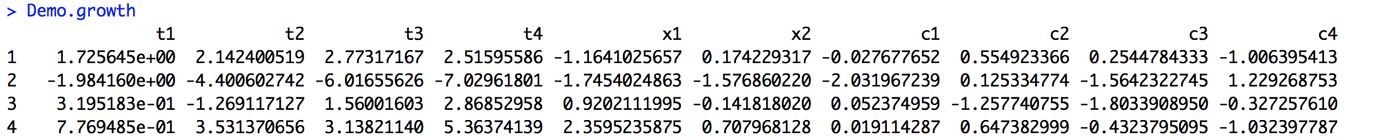
在以下例子中,我們使用人工數據Demo.growth(),包含4個時間點。為了在4個時間點上擬合線性增長模型,我們需要用到含有一個隨機截距潛變數和一個隨機斜率潛變數的模型。
模型如下:
# linear growth model with 4 timepoints
# intercept and slope with fixed coefficients
 i =~ 1*t1 + 1*t2 + 1*t3 + 1*t4
 s =~ 0*t1 + 1*t2 + 2*t3 + 3*t4
數據格式如下:
代碼如下:
model <- 'i =~ 1*t1 + 1*t2 + 1*t3 + 1*t4
          s =~ 0*t1 + 1*t2 + 2*t3 + 3*t4'
fit <- growth(model, data = Demo.growth)
summary(fit)
結果如下:
lavaan (0.5-23.1097) converged normally after  29 iterations

  Number of observations                           400

  Estimator                                         ML
  Minimum Function Test Statistic                8.069
  Degrees of freedom                                 5
  P-value (Chi-square)                           0.152

Parameter Estimates:

  Information                                 Expected
  Standard Errors                             Standard

Latent Variables:
                   Estimate  Std.Err  z-value  P(>|z|)
  i =~
    t1                1.000
    t2                1.000
    t3                1.000
    t4                1.000
  s =~
    t1                0.000
    t2                1.000
    t3                2.000
    t4                3.000

Covariances:
                   Estimate  Std.Err  z-value  P(>|z|)
  i ~~
    s                 0.618    0.071    8.686    0.000

Intercepts:
                   Estimate  Std.Err  z-value  P(>|z|)
   .t1                0.000
   .t2                0.000
   .t3                0.000
   .t4                0.000
    i                 0.615    0.077    8.007    0.000
    s                 1.006    0.042   24.076    0.000

Variances:
                   Estimate  Std.Err  z-value  P(>|z|)
   .t1                0.595    0.086    6.944    0.000
   .t2                0.676    0.061   11.061    0.000
   .t3                0.635    0.072    8.761    0.000
   .t4                0.508    0.124    4.090    0.000
    i                 1.932    0.173   11.194    0.000
    s                 0.587    0.052   11.336    0.000
從技巧上來看,growth()函數與sem()幾乎相同。但是其自動包含了均值結構假設,並預設觀測截距固定為0,潛變數結局和均值自由估計。現在我們再加入兩個變數x1,x2,發展出以下模型:

代碼如下:
# a linear growth model with a time-varying covariate
model <- '# intercept and slope with fixed coefficients
          i =~ 1*t1 + 1*t2 + 1*t3 + 1*t4
          s =~ 0*t1 + 1*t2 + 2*t3 + 3*t4
          # regressions
          i ~ x1 + x2
          s ~ x1 + x2
          # time-varying covariates
          t1 ~ c1
          t2 ~ c2
          t3 ~ c3
          t4 ~ c4'

fit <- growth(model, data = Demo.growth)
summary(fit)
10. 使用分類變數
對於外生分類變數:直接轉換成虛擬變數。
對於內生分類變數:可以直接處理,目前只有WLS方法可用。
 fit <- cfa(myModel, data = myData,
           ordered=c("item1","item2",
                     "item3","item4"))
11. 將協方差矩陣作為輸入
在沒有完整數據集但有協方差矩陣時可以使用,如下例:
# 輸入協方差矩陣
lower <- '
 11.834
  6.947   9.364
  6.819   5.091  12.532
  4.783   5.028   7.495   9.986
 -3.839  -3.889  -3.841  -3.625  9.610
-21.899 -18.831 -21.748 -18.775 35.522 450.288'

# 用getCov建立完整協方差矩陣,輸出是一個矩陣
wheaton.cov <-
getCov(lower, names = c("anomia67", "powerless67",
                        "anomia71", "powerless71",
                        "education", "sei"))

# 模型描述
wheaton.model <- '
  # latent variables
    ses     =~ education + sei
    alien67 =~ anomia67 + powerless67
    alien71 =~ anomia71 + powerless71
  # regressions
    alien71 ~ alien67 + ses
    alien67 ~ ses
  # correlated residuals
    anomia67 ~~ anomia71
    powerless67 ~~ powerless71'

fit <- sem(wheaton.model,
           sample.cov = wheaton.cov,
           sample.nobs = 932)
summary(fit, standardized = TRUE)
結果如下:
lavaan (0.5-23.1097) converged normally after  73 iterations

  Number of observations                           932

  Estimator                                         ML
  Minimum Function Test Statistic                4.735
  Degrees of freedom                                 4
  P-value (Chi-square)                           0.316

Parameter Estimates:

  Information                                 Expected
  Standard Errors                             Standard

Latent Variables:
                   Estimate  Std.Err  z-value  P(>|z|)   Std.lv  Std.all
  ses =~
    education         1.000                               2.607    0.842
    sei               5.219    0.422   12.364    0.000   13.609    0.642
  alien67 =~
    anomia67          1.000                               2.663    0.774
    powerless67       0.979    0.062   15.895    0.000    2.606    0.852
  alien71 =~
    anomia71          1.000                               2.850    0.805
    powerless71       0.922    0.059   15.498    0.000    2.628    0.832

Regressions:
                   Estimate  Std.Err  z-value  P(>|z|)   Std.lv  Std.all
  alien71 ~
    alien67           0.607    0.051   11.898    0.000    0.567    0.567
    ses              -0.227    0.052   -4.334    0.000   -0.207   -0.207
  alien67 ~
    ses              -0.575    0.056  -10.195    0.000   -0.563   -0.563

Covariances:
                   Estimate  Std.Err  z-value  P(>|z|)   Std.lv  Std.all
 .anomia67 ~~
   .anomia71          1.623    0.314    5.176    0.000    1.623    0.356
 .powerless67 ~~
   .powerless71       0.339    0.261    1.298    0.194    0.339    0.121

Variances:
                   Estimate  Std.Err  z-value  P(>|z|)   Std.lv  Std.all
   .education         2.801    0.507    5.525    0.000    2.801    0.292
   .sei             264.597   18.126   14.597    0.000  264.597    0.588
   .anomia67          4.731    0.453   10.441    0.000    4.731    0.400
   .powerless67       2.563    0.403    6.359    0.000    2.563    0.274
   .anomia71          4.399    0.515    8.542    0.000    4.399    0.351
   .powerless71       3.070    0.434    7.070    0.000    3.070    0.308
    ses               6.798    0.649   10.475    0.000    1.000    1.000
   .alien67           4.841    0.467   10.359    0.000    0.683    0.683
   .alien71           4.083    0.404   10.104    0.000    0.503    0.503
12. 估計方法,標準誤差和缺失值
12.1 估計方法
如果所有數據都是連續的,預設估計方法是最大似然法,還有一些其他方法:
- "GLS": generalized least squares. 只能用於完整數據
- "WLS": weighted least squares (sometimes called ADF estimation). 只能用於完整數據
- "DWLS": diagonally weighted least squares
- "ULS": unweighted least squares
許多估計方法都有“穩健”變體,意味著它們提供穩健標準誤差和縮放的檢驗統計量。例如,對於最大似然,lavaan提供如下穩健變體:
- "MLM": maximum likelihood estimation with robust standard errors and a Satorra-Bentler scaled test statistic. 只能用於完整數據
- "MLMVS": maximum likelihood estimation with robust standard errors and a mean- and variance adjusted test statistic (aka the Satterthwaite approach). 只能用於完整數據
- "MLMV": maximum likelihood estimation with robust standard errors and a mean- and variance adjusted test statistic (using a scale-shifted approach). 只能用於完整數據
- "MLF": for maximum likelihood estimation with standard errors based on the first-order derivatives, and a conventional test statistic. 可以用於完整和非完整數據
- "MLR": maximum likelihood estimation with robust (Huber-White) standard errors and a scaled test statistic that is (asymptotically) equal to the Yuan-Bentler test statistic. 可以用於完整和非完整數據
12.2 最大似然估計
lavaan預設使用有偏樣本協方差矩陣,與Mplus所使用方法相似(“normal”)。我們也可以使用likelihood = "wishart"來使用無偏協方差用以接近EQS, LISREL或AMOS的計算結果(“Wishart”):
fit <- cfa(HS.model,
           data = HolzingerSwineford1939,
fit
12.3 缺失值
預設為列表狀態刪除,在進行統計量的計算時,把含有缺失值的記錄刪除,這種方法可以用於計算全體無缺失值數據的均數、協方差和標準差。
13. 間接效應和中介分析
設想一個典型的中介分析,X->M->Y,隨機生成人工數據,示例如下:
set.seed(1234)
X <- rnorm(100)
M <- 0.5*X + rnorm(100)
Y <- 0.7*M + rnorm(100)
Data <- data.frame(X = X, Y = Y, M = M)
model <- '# direct effect
            Y ~ c*X
          # mediator
            M ~ a*X
            Y ~ b*M
          # indirect effect (a*b)
            ab := a*b
          # total effect
            total := c + (a*b)'

fit <- sem(model, data = Data)
summary(fit)
結果如下:
lavaan (0.5-23.1097) converged normally after  12 iterations

  Number of observations                           100

  Estimator                                         ML
  Minimum Function Test Statistic                0.000
  Degrees of freedom                                 0
  Minimum Function Value               0.0000000000000

Parameter Estimates:

  Information                                 Expected
  Standard Errors                             Standard

Regressions:
                   Estimate  Std.Err  z-value  P(>|z|)
  Y ~
    X          (c)    0.036    0.104    0.348    0.728
  M ~
    X          (a)    0.474    0.103    4.613    0.000
  Y ~
    M          (b)    0.788    0.092    8.539    0.000

Variances:
                   Estimate  Std.Err  z-value  P(>|z|)
   .Y                 0.898    0.127    7.071    0.000
   .M                 1.054    0.149    7.071    0.000

Defined Parameters:
                   Estimate  Std.Err  z-value  P(>|z|)
    ab                0.374    0.092    4.059    0.000
    total             0.410    0.125    3.287    0.001
14. 修正指標
可以通過在summary()函數中增加參數modindices = TRUE,來得出修正指標,例如:
fit <- cfa(HS.model,
           data = HolzingerSwineford1939)
mi <- modindices(fit)
mi[mi$op == "=~",]
結果為:
       lhs op rhs     mi    epc sepc.lv sepc.all sepc.nox
25  visual =~  x4  1.211  0.077   0.069    0.059    0.059
26  visual =~  x5  7.441 -0.210  -0.189   -0.147   -0.147
27  visual =~  x6  2.843  0.111   0.100    0.092    0.092
28  visual =~  x7 18.631 -0.422  -0.380   -0.349   -0.349
29  visual =~  x8  4.295 -0.210  -0.189   -0.187   -0.187
30  visual =~  x9 36.411  0.577   0.519    0.515    0.515
31 textual =~  x1  8.903  0.350   0.347    0.297    0.297
32 textual =~  x2  0.017 -0.011  -0.011   -0.010   -0.010
33 textual =~  x3  9.151 -0.272  -0.269   -0.238   -0.238
34 textual =~  x7  0.098 -0.021  -0.021   -0.019   -0.019
35 textual =~  x8  3.359 -0.121  -0.120   -0.118   -0.118
36 textual =~  x9  4.796  0.138   0.137    0.136    0.136
37   speed =~  x1  0.014  0.024   0.015    0.013    0.013
38   speed =~  x2  1.580 -0.198  -0.123   -0.105   -0.105
39   speed =~  x3  0.716  0.136   0.084    0.075    0.075
40   speed =~  x4  0.003 -0.005  -0.003   -0.003   -0.003
41   speed =~  x5  0.201 -0.044  -0.027   -0.021   -0.021
42   speed =~  x6  0.273  0.044   0.027    0.025    0.025
再根據MI(一般以4為標準)和EPC值進行調整。
15. 從擬合方程中提取信息
summary():結果概覽
parameterEstimates(fit):參數估計
 fit <- cfa(HS.model, data=HolzingerSwineford1939)
parameterEstimates(fit)
standardizedSolution():標準化參數估計
 fit <- cfa(HS.model, data=HolzingerSwineford1939)
standardizedSolution(fit)
fitted():擬合協方差矩陣和均值向量
 fit <- cfa(HS.model, data=HolzingerSwineford1939)
fitted(fit)
resid():擬合模型殘差,[觀測協方差矩陣/均值向量]和[隱含協方差矩陣/均值向量]的差
 fit <- cfa(HS.model, data=HolzingerSwineford1939)
resid(fit, type="standardized")
fitMeasures():返回所有擬合度量指標
 fit <- cfa(HS.model, data=HolzingerSwineford1939)
fitMeasures(fit)
fitMeasures(fit, "cfi") # 提取某個具體指標,例如cfi
inspect():查看擬合的lavaan對象具體信息