本文介紹基於Python語言中TensorFlow的Keras介面，實現深度神經網路回歸的方法。 1 寫在前面前期一篇文章Python TensorFlow深度學習回歸代碼：DNNRegressor詳細介紹了基於TensorFlow tf.estimator介面的深度學習網路；而在TensorFl ...

本文介紹基於Python語言中TensorFlow的Keras介面，實現深度神經網路回歸的方法。

1 寫在前面

前期一篇文章Python TensorFlow深度學習回歸代碼：DNNRegressor詳細介紹了基於TensorFlow tf.estimator介面的深度學習網路；而在TensorFlow 2.0中，新的Keras介面具有與 tf.estimator介面一致的功能，且其更易於學習，對於新手而言友好程度更高；在TensorFlow官網也建議新手從Keras介面入手開始學習。因此，本文結合TensorFlow Keras介面，加以深度學習回歸的詳細介紹與代碼實戰。

和上述博客類似，本文第二部分為代碼的分解介紹，第三部分為完整代碼。一些在上述博客介紹過的內容，在本文中就省略了，大家如果有需要可以先查看上述文章Python TensorFlow深度學習回歸代碼：DNNRegressor。

相關版本信息：Python版本：3.8.5；TensorFlow版本：2.4.1；編譯器版本：Spyder 4.1.5。

2 代碼分解介紹

2.1 準備工作

首先需要引入相關的庫與包。

import os
import glob
import openpyxl
import numpy as np
import pandas as pd
import seaborn as sns
import tensorflow as tf
import scipy.stats as stats
import matplotlib.pyplot as plt
from sklearn import metrics
from tensorflow import keras
from tensorflow.keras import layers
from tensorflow.keras import regularizers
from tensorflow.keras.callbacks import ModelCheckpoint
from tensorflow.keras.layers.experimental import preprocessing

由於後續代碼執行過程中，會有很多數據的展示與輸出，其中多數數據都帶有小數部分；為了讓程式所顯示的數據更為整齊、規範，我們可以對代碼的浮點數、數組與NumPy對象對應的顯示規則加以約束。

np.set_printoptions(precision=4,suppress=True)

其中，precision設置小數點後顯示的位數，預設為8；suppress表示是否使用定點計數法（即與科學計數法相對）。

2.2 參數配置

深度學習代碼一大特點即為具有較多的參數需要我們手動定義。為避免調參時上下翻找，我們可以將主要的參數集中在一起，方便我們後期調整。

其中，具體參數的含義在本文後續部分詳細介紹。

# Input parameters.
DataPath="G:/CropYield/03_DL/00_Data/AllDataAll.csv"
ModelPath="G:/CropYield/03_DL/02_DNNModle"
CheckPointPath="G:/CropYield/03_DL/02_DNNModle/Weights"
CheckPointName=CheckPointPath+"/Weights_{epoch:03d}_{val_loss:.4f}.hdf5"
ParameterPath="G:/CropYield/03_DL/03_OtherResult/ParameterResult.xlsx"
TrainFrac=0.8
RandomSeed=np.random.randint(low=21,high=22)
CheckPointMethod='val_loss'
HiddenLayer=[64,128,256,512,512,1024,1024]
RegularizationFactor=0.0001
ActivationMethod='relu'
DropoutValue=[0.5,0.5,0.5,0.3,0.3,0.3,0.2]
OutputLayerActMethod='linear'
LossMethod='mean_absolute_error'
LearnRate=0.005
LearnDecay=0.0005
FitEpoch=500
BatchSize=9999
ValFrac=0.2
BestEpochOptMethod='adam'

2.3 數據導入與數據劃分

我的數據已經保存在了.csv文件中，因此可以用pd.read_csv直接讀取。

其中，數據的每一列是一個特征，每一行是全部特征與因變數（就是下麵的Yield）組合成的樣本。

# Fetch and divide data.
MyData=pd.read_csv(DataPath,names=['EVI0610','EVI0626','EVI0712','EVI0728','EVI0813','EVI0829',
                                   'EVI0914','EVI0930','EVI1016','Lrad06','Lrad07','Lrad08',
                                   'Lrad09','Lrad10','Prec06','Prec07','Prec08','Prec09',
                                   'Prec10','Pres06','Pres07','Pres08','Pres09','Pres10',
                                   'SIF161','SIF177','SIF193','SIF209','SIF225','SIF241',
                                   'SIF257','SIF273','SIF289','Shum06','Shum07','Shum08',
                                   'Shum09','Shum10','SoilType','Srad06','Srad07','Srad08',
                                   'Srad09','Srad10','Temp06','Temp07','Temp08','Temp09',
                                   'Temp10','Wind06','Wind07','Wind08','Wind09','Wind10',
                                   'Yield'],header=0)

隨後，對導入的數據劃分訓練集與測試集。

TrainData=MyData.sample(frac=TrainFrac,random_state=RandomSeed)
TestData=MyData.drop(TrainData.index)

其中，TrainFrac為訓練集（包括驗證數據）所占比例，RandomSeed為隨即劃分數據時所用的隨機數種子。

2.4 聯合分佈圖繪製

在開始深度學習前，我們可以分別對輸入數據的不同特征與因變數的關係加以查看。繪製聯合分佈圖就是一種比較好的查看多個變數之間關係的方法。我們用seaborn來實現這一過程。seaborn是一個基於matplotlib的Python數據可視化庫，使得我們可以通過較為簡單的操作，繪製出動人的圖片。代碼如下：

# Draw the joint distribution image.
def JointDistribution(Factors):
    plt.figure(1)
    sns.pairplot(TrainData[Factors],kind='reg',diag_kind='kde')
    sns.set(font_scale=2.0)
    DataDistribution=TrainData.describe().transpose()
    
# Draw the joint distribution image.
JointFactor=['Lrad07','Prec06','SIF161','Shum06','Srad07','Srad08','Srad10','Temp06','Yield']
JointDistribution(JointFactor)

其中，JointFactor為需要繪製聯合分佈圖的特征名稱，JointDistribution函數中的kind表示聯合分佈圖中非對角線圖的類型，可選'reg'與'scatter'、'kde'、'hist'，'reg'代表在圖片中加入一條擬合直線，'scatter'就是不加入這條直線,'kde'是等高線的形式，'hist'就是類似於柵格地圖的形式；diag_kind表示聯合分佈圖中對角線圖的類型，可選'hist'與'kde'，'hist'代表直方圖，'kde'代表直方圖曲線化。font_scale是圖中的字體大小。JointDistribution函數中最後一句是用來展示TrainData中每一項特征數據的統計信息，包括最大值、最小值、平均值、分位數等。

圖片繪製的示例如下：

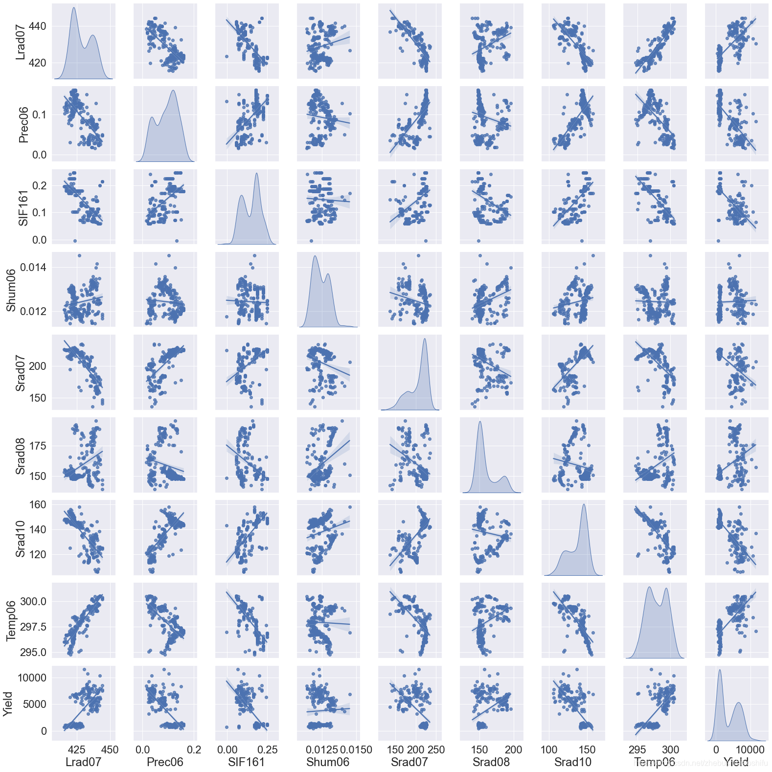
要註意，繪製聯合分佈圖比較慢，建議大家不要選取太多的變數，否則程式會卡在這裡比較長的時間。

2.5 因變數分離與數據標準化

因變數分離我們就不再多解釋啦；接下來，我們要知道，對於機器學習、深度學習而言，數據標準化是十分重要的——用官網所舉的一個例子：不同的特征在神經網路中會乘以相同的權重weight，因此輸入數據的尺度（即數據不同特征之間的大小關係）將會影響到輸出數據與梯度的尺度；因此，數據標準化可以使得模型更加穩定。

在這裡，首先說明數據標準化與歸一化的區別。

標準化即將訓練集中某列的值縮放成均值為0，方差為1的狀態；而歸一化是將訓練集中某列的值縮放到0和1之間。而在機器學習中，標準化較之歸一化通常具有更高的使用頻率，且標準化後的數據在神經網路訓練時，其收斂將會更快。

最後，一定要記得——標準化時只需要對訓練集數據加以處理，不要把測試集Test的數據引入了！因為標準化只需要對訓練數據加以處理，引入測試集反而會影響標準化的作用。

# Separate independent and dependent variables.
TrainX=TrainData.copy(deep=True)
TestX=TestData.copy(deep=True)
TrainY=TrainX.pop('Yield')
TestY=TestX.pop('Yield')

# Standardization data.
Normalizer=preprocessing.Normalization()
Normalizer.adapt(np.array(TrainX))

在這裡，我們直接運用preprocessing.Normalization()建立一個預處理層，其具有數據標準化的功能；隨後，通過.adapt()函數將需要標準化的數據（即訓練集的自變數）放入這一層，便可以實現數據的標準化操作。

2.6 原有模型刪除

我們的程式每執行一次，便會在指定路徑中保存當前運行的模型。為保證下一次模型保存時不受上一次模型運行結果干擾，我們可以將模型文件夾內的全部文件刪除。

# Delete the model result from the last run.
def DeleteOldModel(ModelPath):
    AllFileName=os.listdir(ModelPath)
    for i in AllFileName:
        NewPath=os.path.join(ModelPath,i)
        if os.path.isdir(NewPath):
            DeleteOldModel(NewPath)
        else:
            os.remove(NewPath)
          
# Delete the model result from the last run.
DeleteOldModel(ModelPath)

這一部分的代碼在文章Python TensorFlow深度學習回歸代碼：DNNRegressor有詳細的講解，這裡就不再重覆。

2.7 最優Epoch保存與讀取

在我們訓練模型的過程中，會讓模型運行幾百個Epoch（一個Epoch即全部訓練集數據樣本均進入模型訓練一次）；而由於每一次的Epoch所得到的精度都不一樣，那麼我們自然需要挑出幾百個Epoch中最優秀的那一個Epoch。

# Find and save optimal epoch.
def CheckPoint(Name):
    Checkpoint=ModelCheckpoint(Name,
                               monitor=CheckPointMethod,
                               verbose=1,
                               save_best_only=True,
                               mode='auto')
    CallBackList=[Checkpoint]
    return CallBackList

# Find and save optimal epochs.
CallBack=CheckPoint(CheckPointName)

其中，Name就是保存Epoch的路徑與文件名命名方法；monitor是我們挑選最優Epoch的依據，在這裡我們用驗證集數據對應的誤差來判斷這個Epoch是不是我們想要的；verbose用來設置輸出日誌的內容，我們用1就好；save_best_only用來確定我們是否只保存被認定為最優的Epoch；mode用以判斷我們的monitor是越大越好還是越小越好，前面提到了我們的monitor是驗證集數據對應的誤差，那麼肯定是誤差越小越好，所以這裡可以用'auto'或'min'，其中'auto'是模型自己根據用戶選擇的monitor方法來判斷越大越好還是越小越好。

找到最優Epoch後，將其傳遞給CallBack。需要註意的是，這裡的最優Epoch是多個Epoch——因為每一次Epoch只要獲得了當前模型所遇到的最優解，它就會保存；下一次再遇見一個更好的解時，同樣保存，且不覆蓋上一次的Epoch。可以這麼理解，假如一共有三次Epoch，所得到的誤差分別為5，7，4；那麼我們保存的Epoch就是第一次和第三次。

2.8 模型構建

Keras介面下的模型構建就很清晰明瞭了。相信大家在看了前期一篇文章Python TensorFlow深度學習回歸代碼：DNNRegressor後，結合代碼旁的註釋就理解啦。

# Build DNN model.
def BuildModel(Norm):
    Model=keras.Sequential([Norm, # 數據標準化層
                            
                            layers.Dense(HiddenLayer[0], # 指定隱藏層1的神經元個數
                                         kernel_regularizer=regularizers.l2(RegularizationFactor), # 運用L2正則化
                                         # activation=ActivationMethod
                                         ),
                            layers.LeakyReLU(), # 引入LeakyReLU這一改良的ReLU激活函數，從而加快模型收斂，減少過擬合
                            layers.BatchNormalization(), # 引入Batch Normalizing，加快網路收斂與增強網路穩固性
                            layers.Dropout(DropoutValue[0]), # 指定隱藏層1的Dropout值
                            
                            layers.Dense(HiddenLayer[1],
                                         kernel_regularizer=regularizers.l2(RegularizationFactor),
                                         # activation=ActivationMethod
                                         ),
                            layers.LeakyReLU(),
                            layers.BatchNormalization(),
                            layers.Dropout(DropoutValue[1]),
                            
                            layers.Dense(HiddenLayer[2],
                                         kernel_regularizer=regularizers.l2(RegularizationFactor),
                                         # activation=ActivationMethod
                                         ),
                            layers.LeakyReLU(),
                            layers.BatchNormalization(),
                            layers.Dropout(DropoutValue[2]),
                            
                            layers.Dense(HiddenLayer[3],
                                         kernel_regularizer=regularizers.l2(RegularizationFactor),
                                         # activation=ActivationMethod
                                         ),
                            layers.LeakyReLU(),
                            layers.BatchNormalization(),
                            layers.Dropout(DropoutValue[3]),
                            
                            layers.Dense(HiddenLayer[4],
                                         kernel_regularizer=regularizers.l2(RegularizationFactor),
                                         # activation=ActivationMethod
                                         ),
                            layers.LeakyReLU(),
                            layers.BatchNormalization(),
                            layers.Dropout(DropoutValue[4]),
                            
                            layers.Dense(HiddenLayer[5],
                                         kernel_regularizer=regularizers.l2(RegularizationFactor),
                                         # activation=ActivationMethod
                                         ),
                            layers.LeakyReLU(),
                            layers.BatchNormalization(),
                            layers.Dropout(DropoutValue[5]),
                            
                            layers.Dense(HiddenLayer[6],
                                         kernel_regularizer=regularizers.l2(RegularizationFactor),
                                         # activation=ActivationMethod
                                         ),
                            layers.LeakyReLU(),
                            # If batch normalization is set in the last hidden layer, the error image
                            # will show a trend of first stable and then decline; otherwise, it will 
                            # decline and then stable.
                            # layers.BatchNormalization(),
                            layers.Dropout(DropoutValue[6]),
                            
                            layers.Dense(units=1,
                                         activation=OutputLayerActMethod)]) # 最後一層就是輸出層
    Model.compile(loss=LossMethod, # 指定每個批次訓練誤差的減小方法
                  optimizer=tf.keras.optimizers.Adam(learning_rate=LearnRate,decay=LearnDecay)) 
                  # 運用學習率下降的優化方法
    return Model
   
# Build DNN regression model.
DNNModel=BuildModel(Normalizer)
DNNModel.summary()
DNNHistory=DNNModel.fit(TrainX,
                        TrainY,
                        epochs=FitEpoch,
                        # batch_size=BatchSize,
                        verbose=1,
                        callbacks=CallBack,
                        validation_split=ValFrac)

在這裡，.summary()查看模型摘要，validation_split為在訓練數據中，取出ValFrac所指定比例的一部分作為驗證數據。DNNHistory則記錄了模型訓練過程中的各類指標變化情況，接下來我們可以基於其繪製模型訓練過程的誤差變化圖像。

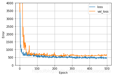
2.9 訓練圖像繪製

機器學習中，過擬合是影響訓練精度的重要因素。因此，我們最好在訓練模型的過程中繪製訓練數據、驗證數據的誤差變化圖象，從而更好獲取模型的訓練情況。

# Draw error image.
def LossPlot(History):
    plt.figure(2)
    plt.plot(History.history['loss'],label='loss')
    plt.plot(History.history['val_loss'],label='val_loss')
    plt.ylim([0,4000])
    plt.xlabel('Epoch')
    plt.ylabel('Error')
    plt.legend()
    plt.grid(True)

# Draw error image.
LossPlot(DNNHistory)

其中，'loss'與'val_loss'分別是模型訓練過程中，訓練集、驗證集對應的誤差；如果訓練集誤差明顯小於驗證集誤差，就說明模型出現了過擬合。

2.10 最優Epoch選取

前面提到了，我們將多個符合要求的Epoch保存在了指定的路徑下，那麼最終我們可以從中選取最好的那個Epoch，作為模型的最終參數，從而對測試集數據加以預測。那麼在這裡，我們需要將這一全局最優Epoch選取出，並帶入到最終的模型里。

# Optimize the model based on optimal epoch.
def BestEpochIntoModel(Path,Model):
    EpochFile=glob.glob(Path+'/*')
    BestEpoch=max(EpochFile,key=os.path.getmtime)
    Model.load_weights(BestEpoch)
    Model.compile(loss=LossMethod,
                  optimizer=BestEpochOptMethod)
    return Model

# Optimize the model based on optimal epoch.
DNNModel=BestEpochIntoModel(CheckPointPath,DNNModel）

總的來說，這裡就是運用了os.path.getmtime模塊，將我們存儲Epoch的文件夾中最新的那個Epoch挑出來——這一Epoch就是使得驗證集數據誤差最小的全局最優Epoch；並通過load_weights將這一Epoch對應的模型參數引入模型。

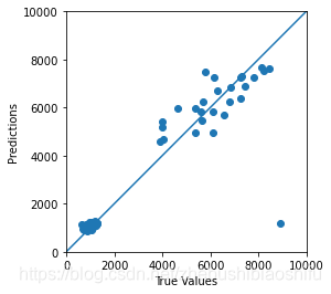
2.11 模型測試、擬合圖像繪製、精度驗證與模型參數與結果保存

前期一篇文章Python TensorFlow深度學習回歸代碼：DNNRegressor中有相關的代碼講解內容，因此這裡就不再贅述啦。

# Draw Test image.
def TestPlot(TestY,TestPrediction):
    plt.figure(3)
    ax=plt.axes(aspect='equal')
    plt.scatter(TestY,TestPrediction)
    plt.xlabel('True Values')
    plt.ylabel('Predictions')
    Lims=[0,10000]
    plt.xlim(Lims)
    plt.ylim(Lims)
    plt.plot(Lims,Lims)
    plt.grid(False)

# Verify the accuracy and draw error hist image.
def AccuracyVerification(TestY,TestPrediction):
    DNNError=TestPrediction-TestY
    plt.figure(4)
    plt.hist(DNNError,bins=30)
    plt.xlabel('Prediction Error')
    plt.ylabel('Count')
    plt.grid(False)
    Pearsonr=stats.pearsonr(TestY,TestPrediction)
    R2=metrics.r2_score(TestY,TestPrediction)
    RMSE=metrics.mean_squared_error(TestY,TestPrediction)**0.5
    print('Pearson correlation coefficient is {0}, and RMSE is {1}.'.format(Pearsonr[0],RMSE))
    return (Pearsonr[0],R2,RMSE)

# Save key parameters.
def WriteAccuracy(*WriteVar):
    ExcelData=openpyxl.load_workbook(WriteVar[0])
    SheetName=ExcelData.get_sheet_names()
    WriteSheet=ExcelData.get_sheet_by_name(SheetName[0])
    WriteSheet=ExcelData.active
    MaxRowNum=WriteSheet.max_row
    for i in range(len(WriteVar)-1):
        exec("WriteSheet.cell(MaxRowNum+1,i+1).value=WriteVar[i+1]")
    ExcelData.save(WriteVar[0])

# Predict test set data.
TestPrediction=DNNModel.predict(TestX).flatten()

# Draw Test image.
TestPlot(TestY,TestPrediction)

# Verify the accuracy and draw error hist image.
AccuracyResult=AccuracyVerification(TestY,TestPrediction)
PearsonR,R2,RMSE=AccuracyResult[0],AccuracyResult[1],AccuracyResult[2]

# Save model and key parameters.
DNNModel.save(ModelPath)
WriteAccuracy(ParameterPath,PearsonR,R2,RMSE,TrainFrac,RandomSeed,CheckPointMethod,
              ','.join('%s' %i for i in HiddenLayer),RegularizationFactor,
              ActivationMethod,','.join('%s' %i for i in DropoutValue),OutputLayerActMethod,
              LossMethod,LearnRate,LearnDecay,FitEpoch,BatchSize,ValFrac,BestEpochOptMethod)

得到擬合圖像如下：

得到誤差分佈直方圖如下：

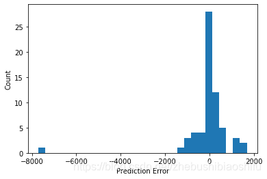
至此，代碼的分解介紹就結束啦~

3 完整代碼

# -*- coding: utf-8 -*-
"""
Created on Tue Feb 24 12:42:17 2021

@author: fkxxgis
"""

import os
import glob
import openpyxl
import numpy as np
import pandas as pd
import seaborn as sns
import tensorflow as tf
import scipy.stats as stats
import matplotlib.pyplot as plt
from sklearn import metrics
from tensorflow import keras
from tensorflow.keras import layers
from tensorflow.keras import regularizers
from tensorflow.keras.callbacks import ModelCheckpoint
from tensorflow.keras.layers.experimental import preprocessing

np.set_printoptions(precision=4,suppress=True)

# Draw the joint distribution image.
def JointDistribution(Factors):
    plt.figure(1)
    sns.pairplot(TrainData[Factors],kind='reg',diag_kind='kde')
    sns.set(font_scale=2.0)
    DataDistribution=TrainData.describe().transpose()

# Delete the model result from the last run.
def DeleteOldModel(ModelPath):
    AllFileName=os.listdir(ModelPath)
    for i in AllFileName:
        NewPath=os.path.join(ModelPath,i)
        if os.path.isdir(NewPath):
            DeleteOldModel(NewPath)
        else:
            os.remove(NewPath)

# Find and save optimal epoch.
def CheckPoint(Name):
    Checkpoint=ModelCheckpoint(Name,
                               monitor=CheckPointMethod,
                               verbose=1,
                               save_best_only=True,
                               mode='auto')
    CallBackList=[Checkpoint]
    return CallBackList

# Build DNN model.
def BuildModel(Norm):
    Model=keras.Sequential([Norm, # 數據標準化層
                            
                            layers.Dense(HiddenLayer[0], # 指定隱藏層1的神經元個數
                                         kernel_regularizer=regularizers.l2(RegularizationFactor), # 運用L2正則化
                                         # activation=ActivationMethod
                                         ),
                            layers.LeakyReLU(), # 引入LeakyReLU這一改良的ReLU激活函數，從而加快模型收斂，減少過擬合
                            layers.BatchNormalization(), # 引入Batch Normalizing，加快網路收斂與增強網路穩固性
                            layers.Dropout(DropoutValue[0]), # 指定隱藏層1的Dropout值
                            
                            layers.Dense(HiddenLayer[1],
                                         kernel_regularizer=regularizers.l2(RegularizationFactor),
                                         # activation=ActivationMethod
                                         ),
                            layers.LeakyReLU(),
                            layers.BatchNormalization(),
                            layers.Dropout(DropoutValue[1]),
                            
                            layers.Dense(HiddenLayer[2],
                                         kernel_regularizer=regularizers.l2(RegularizationFactor),
                                         # activation=ActivationMethod
                                         ),
                            layers.LeakyReLU(),
                            layers.BatchNormalization(),
                            layers.Dropout(DropoutValue[2]),
                            
                            layers.Dense(HiddenLayer[3],
                                         kernel_regularizer=regularizers.l2(RegularizationFactor),
                                         # activation=ActivationMethod
                                         ),
                            layers.LeakyReLU(),
                            layers.BatchNormalization(),
                            layers.Dropout(DropoutValue[3]),
                            
                            layers.Dense(HiddenLayer[4],
                                         kernel_regularizer=regularizers.l2(RegularizationFactor),
                                         # activation=ActivationMethod
                                         ),
                            layers.LeakyReLU(),
                            layers.BatchNormalization(),
                            layers.Dropout(DropoutValue[4]),
                            
                            layers.Dense(HiddenLayer[5],
                                         kernel_regularizer=regularizers.l2(RegularizationFactor),
                                         # activation=ActivationMethod
                                         ),
                            layers.LeakyReLU(),
                            layers.BatchNormalization(),
                            layers.Dropout(DropoutValue[5]),
                            
                            layers.Dense(HiddenLayer[6],
                                         kernel_regularizer=regularizers.l2(RegularizationFactor),
                                         # activation=ActivationMethod
                                         ),
                            layers.LeakyReLU(),
                            # If batch normalization is set in the last hidden layer, the error image
                            # will show a trend of first stable and then decline; otherwise, it will 
                            # decline and then stable.
                            # layers.BatchNormalization(),
                            layers.Dropout(DropoutValue[6]),
                            
                            layers.Dense(units=1,
                                         activation=OutputLayerActMethod)]) # 最後一層就是輸出層
    Model.compile(loss=LossMethod, # 指定每個批次訓練誤差的減小方法
                  optimizer=tf.keras.optimizers.Adam(learning_rate=LearnRate,decay=LearnDecay)) 
                  # 運用學習率下降的優化方法
    return Model

# Draw error image.
def LossPlot(History):
    plt.figure(2)
    plt.plot(History.history['loss'],label='loss')
    plt.plot(History.history['val_loss'],label='val_loss')
    plt.ylim([0,4000])
    plt.xlabel('Epoch')
    plt.ylabel('Error')
    plt.legend()
    plt.grid(True)

# Optimize the model based on optimal epoch.
def BestEpochIntoModel(Path,Model):
    EpochFile=glob.glob(Path+'/*')
    BestEpoch=max(EpochFile,key=os.path.getmtime)
    Model.load_weights(BestEpoch)
    Model.compile(loss=LossMethod,
                  optimizer=BestEpochOptMethod)
    return Model

# Draw Test image.
def TestPlot(TestY,TestPrediction):
    plt.figure(3)
    ax=plt.axes(aspect='equal')
    plt.scatter(TestY,TestPrediction)
    plt.xlabel('True Values')
    plt.ylabel('Predictions')
    Lims=[0,10000]
    plt.xlim(Lims)
    plt.ylim(Lims)
    plt.plot(Lims,Lims)
    plt.grid(False)

# Verify the accuracy and draw error hist image.
def AccuracyVerification(TestY,TestPrediction):
    DNNError=TestPrediction-TestY
    plt.figure(4)
    plt.hist(DNNError,bins=30)
    plt.xlabel('Prediction Error')
    plt.ylabel('Count')
    plt.grid(False)
    Pearsonr=stats.pearsonr(TestY,TestPrediction)
    R2=metrics.r2_score(TestY,TestPrediction)
    RMSE=metrics.mean_squared_error(TestY,TestPrediction)**0.5
    print('Pearson correlation coefficient is {0}, and RMSE is {1}.'.format(Pearsonr[0],RMSE))
    return (Pearsonr[0],R2,RMSE)

# Save key parameters.
def WriteAccuracy(*WriteVar):
    ExcelData=openpyxl.load_workbook(WriteVar[0])
    SheetName=ExcelData.get_sheet_names()
    WriteSheet=ExcelData.get_sheet_by_name(SheetName[0])
    WriteSheet=ExcelData.active
    MaxRowNum=WriteSheet.max_row
    for i in range(len(WriteVar)-1):
        exec("WriteSheet.cell(MaxRowNum+1,i+1).value=WriteVar[i+1]")
    ExcelData.save(WriteVar[0])

# Input parameters.
DataPath="G:/CropYield/03_DL/00_Data/AllDataAll.csv"
ModelPath="G:/CropYield/03_DL/02_DNNModle"
CheckPointPath="G:/CropYield/03_DL/02_DNNModle/Weights"
CheckPointName=CheckPointPath+"/Weights_{epoch:03d}_{val_loss:.4f}.hdf5"
ParameterPath="G:/CropYield/03_DL/03_OtherResult/ParameterResult.xlsx"
TrainFrac=0.8
RandomSeed=np.random.randint(low=21,high=22)
CheckPointMethod='val_loss'
HiddenLayer=[64,128,256,512,512,1024,1024]
RegularizationFactor=0.0001
ActivationMethod='relu'
DropoutValue=[0.5,0.5,0.5,0.3,0.3,0.3,0.2]
OutputLayerActMethod='linear'
LossMethod='mean_absolute_error'
LearnRate=0.005
LearnDecay=0.0005
FitEpoch=500
BatchSize=9999
ValFrac=0.2
BestEpochOptMethod='adam'

# Fetch and divide data.
MyData=pd.read_csv(DataPath,names=['EVI0610','EVI0626','EVI0712','EVI0728','EVI0813','EVI0829',
                                   'EVI0914','EVI0930','EVI1016','Lrad06','Lrad07','Lrad08',
                                   'Lrad09','Lrad10','Prec06','Prec07','Prec08','Prec09',
                                   'Prec10','Pres06','Pres07','Pres08','Pres09','Pres10',
                                   'SIF161','SIF177','SIF193','SIF209','SIF225','SIF241',
                                   'SIF257','SIF273','SIF289','Shum06','Shum07','Shum08',
                                   'Shum09','Shum10','SoilType','Srad06','Srad07','Srad08',
                                   'Srad09','Srad10','Temp06','Temp07','Temp08','Temp09',
                                   'Temp10','Wind06','Wind07','Wind08','Wind09','Wind10',
                                   'Yield'],header=0)
TrainData=MyData.sample(frac=TrainFrac,random_state=RandomSeed)
TestData=MyData.drop(TrainData.index)

# Draw the joint distribution image.
# JointFactor=['Lrad07','Prec06','SIF161','Shum06','Srad07','Srad08','Srad10','Temp06','Yield']
# JointDistribution(JointFactor)

# Separate independent and dependent variables.
TrainX=TrainData.copy(deep=True)
TestX=TestData.copy(deep=True)
TrainY=TrainX.pop('Yield')
TestY=TestX.pop('Yield')

# Standardization data.
Normalizer=preprocessing.Normalization()
Normalizer.adapt(np.array(TrainX))

# Delete the model result from the last run.
DeleteOldModel(ModelPath)

# Find and save optimal epochs.
CallBack=CheckPoint(CheckPointName)

# Build DNN regression model.
DNNModel=BuildModel(Normalizer)
DNNModel.summary()
DNNHistory=DNNModel.fit(TrainX,
                        TrainY,
                        epochs=FitEpoch,
                        # batch_size=BatchSize,
                        verbose=1,
                        callbacks=CallBack,
                        validation_split=ValFrac)

# Draw error image.
LossPlot(DNNHistory)

# Optimize the model based on optimal epoch.
DNNModel=BestEpochIntoModel(CheckPointPath,DNNModel)

# Predict test set data.
TestPrediction=DNNModel.predict(TestX).flatten()

# Draw Test image.
TestPlot(TestY,TestPrediction)

# Verify the accuracy and draw error hist image.
AccuracyResult=AccuracyVerification(TestY,TestPrediction)
PearsonR,R2,RMSE=AccuracyResult[0],AccuracyResult[1],AccuracyResult[2]

# Save model and key parameters.
DNNModel.save(ModelPath)
WriteAccuracy(ParameterPath,PearsonR,R2,RMSE,TrainFrac,RandomSeed,CheckPointMethod,
              ','.join('%s' %i for i in HiddenLayer),RegularizationFactor,
              ActivationMethod,','.join('%s' %i for i in DropoutValue),OutputLayerActMethod,
              LossMethod,LearnRate,LearnDecay,FitEpoch,BatchSize,ValFrac,BestEpochOptMethod)

至此，大功告成。

Python TensorFlow深度神經網路回歸：keras.Sequential